A few years ago, I noticed a trending Reddit “LifePro Tip” challenging people to reimagine the price of items purchased (especially impulse items) into the hours spent working to afford them.
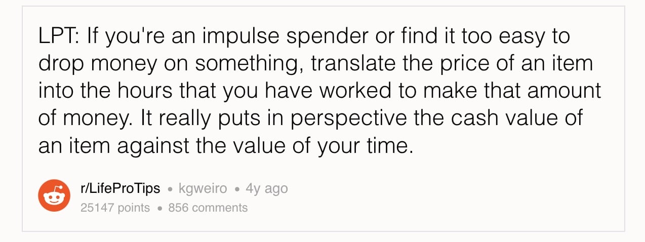
The idea isn’t to make you feel guilty, but rather to encourage mindful spending and intentional consumption.
Seeing the cost of everything you buy translated into the hours of your life exchanged to afford them instantly puts spending into perspective.
Henry Thoreau knew this 170 years ago:
“The cost of a thing is the amount of what I will call life which is required to be exchanged for it, immediately or in the long run.”
Thoreau, “Walden”
How to visualize your spending as hours of work
In Google Sheets powered by Tiller, a simple array formula can instantly convert your spending into hours of work based on your hourly pay.
Tiller founder Peter Polson outlines the steps in this older video on YouTube.
You can see how this works with your own hourly wage with this free demo version of the Tiller Foundation Template.
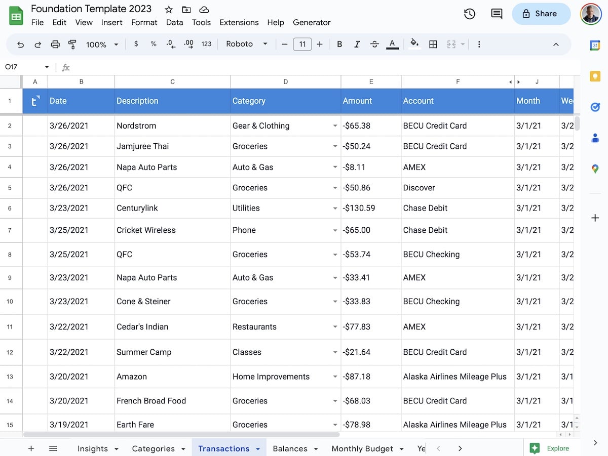
1 – In your Tiller-powered Google Sheet, navigate to your Transactions sheet:
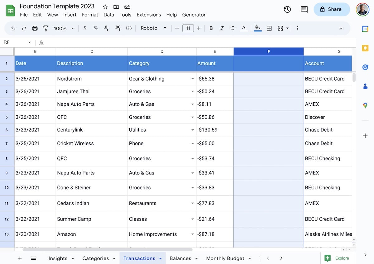
2 – In the example Transactions sheet, add a new column between the “Amount” column and the “Account” column. The new column is column F:
3. In cell F1, add the array formula below:
The array formula is:
=arrayformula(if(row(E:E)=1,"Hours to Earn",(if((D:D)="Credit Card Payment","",(if((E:E)<0,(E:E)/-33,""))))))Paste the formula into cell F1:
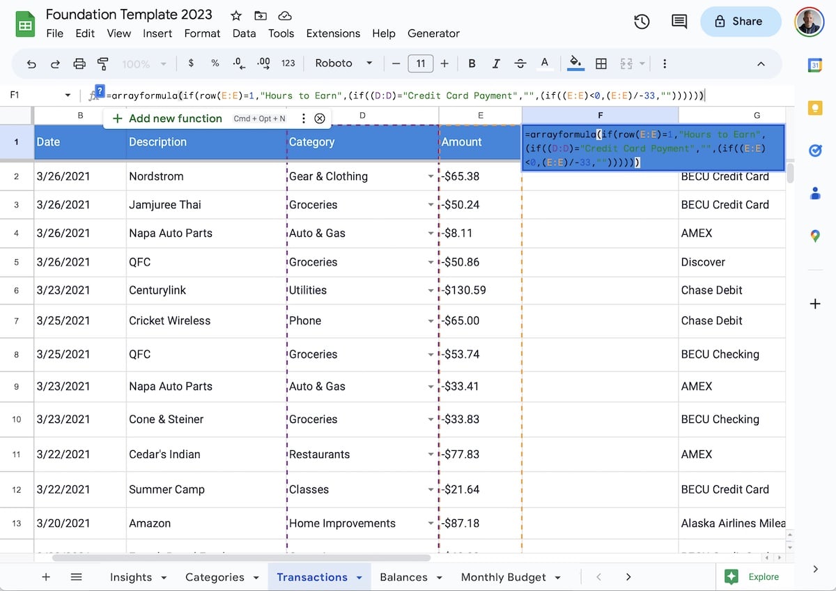
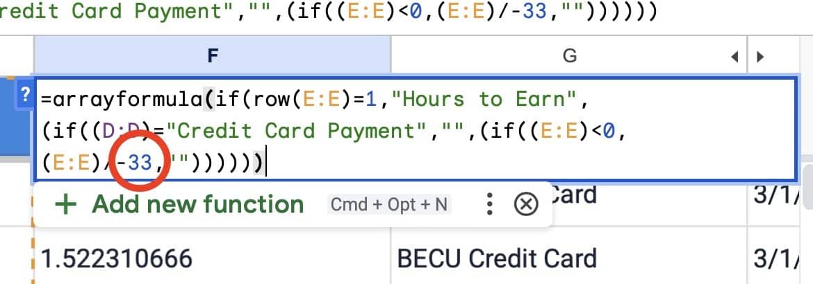
To calculate your hourly wage, it’s best to use your after-tax take-home rate. In the formula above (circled in the image below), the hourly rate is $33.
Modify this number to reflect your actual after-tax earnings:
This array formula will ignore any payments categorized “Credit Card Payment,” in column D, as these are transfers and not expenditures.
It also looks in column E for any payments above one dollar. The array formula will fill the whole column below with data.
You may need to slightly modify the formula to work with your spreadsheet. For example, in your Tiller sheet, if your Amount is not in Column E you’d want to update the formula to reflect that. Same if your Categories aren’t in column D.
Share your thoughts in the Tiller Community
That’s it. It’s a simple yet powerful formula. We’d love to hear what you’ve created in your Tiller sheet that you think others might want to know about. Share your thoughts here in the Tiller Community!
.


